1D Relaxation Analysis

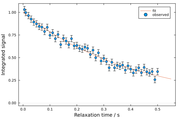
The relaxation analysis module in NMRAnalysis.jl provides a tool for analysing R1 and R2 measurements, fitting either to an exponential decay:

\[I(\tau) = I_0 \exp\left(-R\tau\right)\]

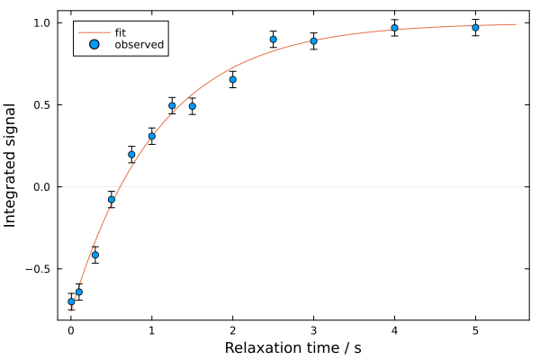
or to an inversion-recovery model:

\[I(\tau) = I_0 \cdot \left[1 - A \exp\left(-R\tau\right)\right]\]

where $I_0$ is the maximum intensity, $R$ is the relaxation rate, and $A$ is the amplitude of the recovery phase.

Required Annotations

The relaxation analysis requires the following annotations in the experiment file:

The experiment must also have types including "1d" and "relaxation", with features including either "R1" or "R2" for automatic dispatch via analyse().

Launching Relaxation Analysis

Automatic Dispatch

The simplest way to analyse a relaxation experiment is using the analyse() function, which automatically detects the experiment type from annotations:

using NMRAnalysis

analyse("path/to/experiment")  # auto-detects and runs appropriate analysis

See Automatic Analysis for how analyse() decides which routine to run.

Direct Call

You can also call relaxation1d() directly:

relaxation1d("path/to/experiment")

Analysis Workflow

1. Region Selection

When launched, the analysis displays the spectrum and prompts you to select integration and noise regions interactively. For inversion-recovery experiments, the last slice (where signal is most recovered) is shown; for exponential decay, the first slice is used.

2. Fitting and Results

After region selection, the fit runs automatically. Results are displayed in the terminal:

[ Info: Relaxation analysis results for /path/to/experiment:
[ Info:  - R1 relaxation of 19F
[ Info:  - Model: Inversion recovery
[ Info:  - Integration region: -63.0 .. -62.5 ppm
[ Info:  - Noise region: -67.25 .. -66.75 ppm
[ Info:  - Fitted relaxation rate: 0.866 ± 0.025 s⁻¹
[ Info:  - Fitted relaxation time: 1.154 ± 0.034 s
[ Info:  - Inversion-recovery amplitude: 1.866 ± 0.025

A fit plot is also displayed:

For inversion-recovery fits, the amplitude parameter is also reported:

3. Return Value

The function returns a named tuple containing:

Noise Estimation

Noise levels for peak integrals are calculated by integrating a matching region of noise and taking the standard deviation across relaxation delays. This approach relies on good quality baselines for accurate noise estimation.