Magnetisation Recovery

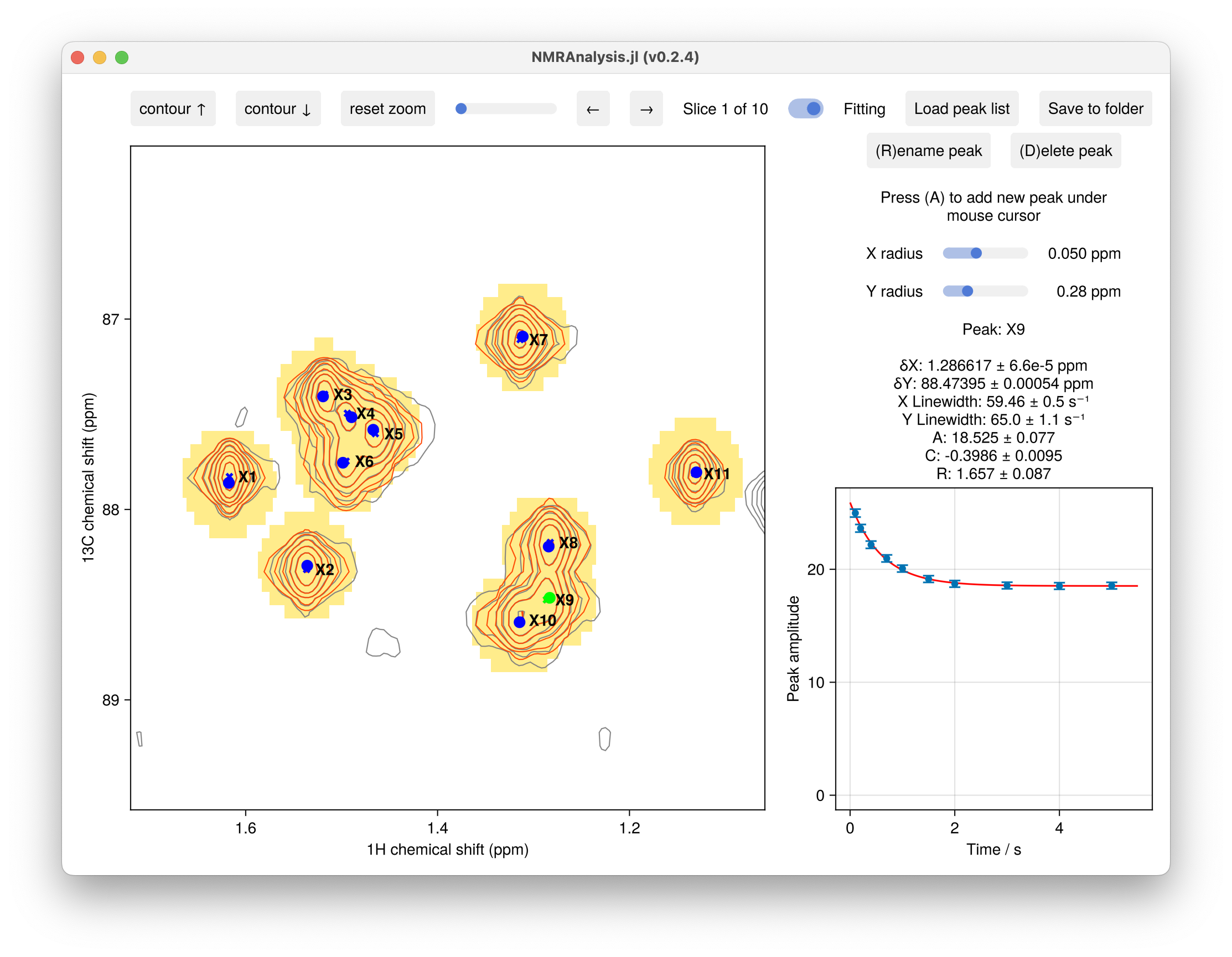
The recovery2d function measures longitudinal relaxation from an inversion recovery or saturation recovery experiment. Peak amplitudes are fitted to a magnetisation recovery model:

\[I(\tau) = A \left(1 - C \exp\!\left(-R\tau\right)\right)\]

where $R$ is the recovery rate (s⁻¹), $A$ is the equilibrium amplitude, and $C$ is the recovery amplitude factor. For an ideal inversion recovery experiment $C = 2$, while for saturation recovery $C = 1$.

Usage

using NMRAnalysis

# Variable delay list
t = [0.1, 0.2, 0.4, 0.7, 1.0, 1.5, 2.0, 3.0, 4.0, 5.0]
recovery2d("33", t)

# Read delays from a file
recovery2d("33", "vdlist.txt")

When the experiment is stored as a pseudo-3D dataset in a single processed directory, a single path string is passed; when each delay is a separate experiment, pass a vector of paths alongside the corresponding delay values.

Output

Clicking Save to folder writes all results to results.csv. Alongside peak positions, linewidths and amplitudes, the derived columns are:

See Peak Lists and Output Files for the full format. Plot R against residue number with summaryplot("results.csv") (or summaryplot("output-folder/").