Pulse Calibration
calibration1d analyses a nutation experiment: a series of spectra recorded with increasing pulse duration, from which the B₁ field strength, the 90° pulse length and the B₁ inhomogeneity follow. This is how spin-lock powers are calibrated before an R1ρ or CEST experiment.
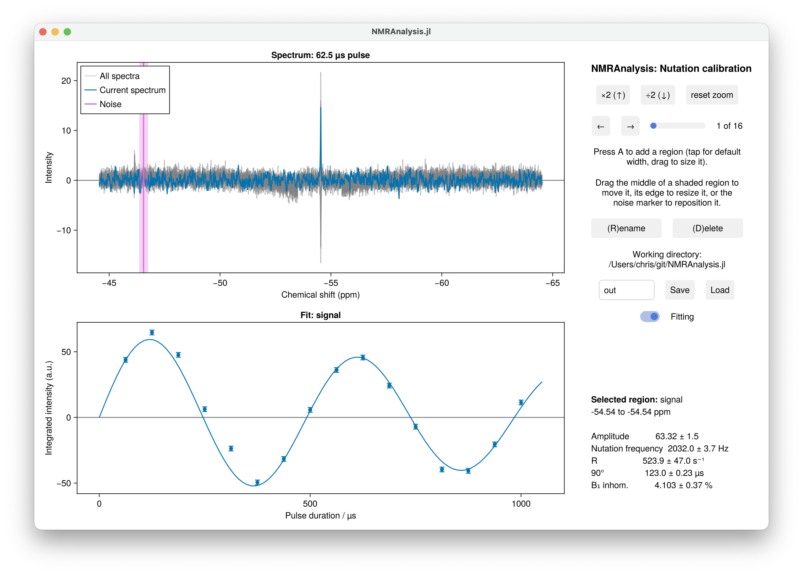
Running the analysis
using NMRAnalysis

results = calibration1d("1")
The analysis window opens with a region on the tallest peak. Check that it sits over the signal you are calibrating on, put the noise marker somewhere empty, and press Save.
Calibrating over several power levels
Give several experiments, recorded at different power levels, and each is fitted separately and the results combined into a calibration curve:
results = calibration1d(["1", "2", "3"])Each power level appears as its own series in the window, and each contributes its own nutation frequency and 90° pulse length. The combined result is reported as nu1ref, the field at the reference power powerref (the first experiment's), and linearity, the fitted exponent of
\[\nu_1(p) = \nu_1^\text{ref} \cdot 10^{-L(\text{dB}(p) - \text{dB}(p_\text{ref}))/20}.\]
A linearity L of 1 means the amplifier follows the ideal ν₁ ∝ √W. Below 1 the field falls short of the ideal law as the power is raised, which is the usual signature of amplifier compression; this is exactly what a single-power calibration cannot see, since it has to assume L = 1.
The power level of each experiment is read from its calibration.power annotation, or you can give them with power=[-18.0, -12.0, -6.0], in dB. A single experiment still calibrates, reporting the field at its own power with the linearity assumed ideal.
Save then writes calibration.pdf alongside the usual output: ν₁ against power on a log axis, where the ideal power law is a straight line, with the fitted curve through the measurements and the residuals from it underneath in percent. Amplifier compression is a percent or two and invisible against a decade of field strength, so the residual panel is where you see it. One power level gets no plot, having no curve to draw.
fit.pdf holds the nutation curves themselves, one panel per power level. They are not drawn on a shared axis: the 90° pulse at the lowest power can be ten times the longest duration sampled at the highest, which would leave the fastest nutation as a spike against the origin.
Using a calibration in other analyses
B1Calibration turns an analysis into the object the exchange analyses take, so that CEST and R1ρ are simulated with measured field strengths and a measured B₁ inhomogeneity rather than nominal ones:
cal = B1Calibration(calibration1d(["1", "2", "3"]))

hz(Power(-15.0, :dB), cal)     # field strength (Hz) at a power you did not calibrate at
Power(2000.0, cal)             # the power to set for a 2 kHz field

exchange1d(["11", "12"]; calibration=cal)
The calibration experiments can also be passed directly, in which case they are fitted without a window opening:
exchange1d(["11", "12"]; calibration=["1", "2", "3"])
setupR1rhopowers(["1", "2", "3"])
A calibration fitted on the way to something else is still a measurement and still needs checking, so when that analysis saves its results the calibration's own analysis is written into a calibration/ folder beside them: the fits in fit.pdf, the curve in calibration.pdf, the numbers in summary.txt and results.csv. An analysis that is never saved leaves nothing behind. To fit a calibration and save it where you choose, use calibrationanalysis, which hands back the calibration and a function that writes it:
cal, save = calibrationanalysis(["1", "2", "3"])
save("mycalibration")
Without a calibration, each experiment falls back to its own reference pulse (p1/pl1) on the assumption of a perfectly linear amplifier, and the B₁ inhomogeneity is taken to be 5%. See B₁ inhomogeneity for how the distribution enters the simulations.
Durations and modulation
The pulse durations and the modulation are found in the usual order of precedence:
| From an argument | From an annotation | Otherwise | |
|---|---|---|---|
| Durations | durations=[1e-5, 2e-5, …], in seconds | calibration.duration | you are asked, in µs |
| Modulation | phase=:sine or :cosine | calibration.model | you choose from a menu |
A sine modulation is the usual case, where the experiment starts from equilibrium; a cosine modulation applies where it starts from transverse magnetisation.
Pulse programme
An annotated ¹⁹F nutation sequence is available at 19f_calib_nut.cw. Its annotations let analyse recognise the experiment and run this analysis without being told which one to use:
analyse("examples/calibration/1")| Annotation | Meaning |
|---|---|
calibration.channel | Channel being calibrated, e.g. "f1" |
calibration.power | Power level used |
calibration.duration | Pulse durations |
calibration.model | "sine_modulated" or "cosine_modulated" |
What is fitted
A sinusoid with a Gaussian envelope,
\[I(t) = A \sin(2\pi \nu t) \exp\left(-\tfrac{1}{2}(2\pi \sigma \nu t)^2\right),\]
or a cosine in place of the sine, from which the 90° pulse length follows as
\[t_{90} = \frac{1}{4\nu}.\]
The envelope is Gaussian rather than exponential because that is what a Gaussian spread of B₁ produces: averaging $\sin(2\pi\nu t)$ over a distribution of ν with mean ν̄ and standard deviation σν̄ gives $\sin(2\pi\bar\nu t)\exp(-\tfrac{1}{2}(2\pi\sigma\bar\nu t)^2)$. Fitting it this way makes σ the width of the B₁ distribution directly, which is the same quantity the CEST and R1ρ simulations sample. It is fitted, and reported, as a percentage.
| Parameter | Meaning |
|---|---|
A | Amplitude |
nu | Nutation frequency, Hz |
sigma | Width of the B₁ distribution at this power level, % |
power | Power level, dB (single-power analyses only) |
pulse90 | 90° pulse length, µs |
inhomogeneity | B₁ inhomogeneity, %: the smallest sigma |
powerref, nu1ref, linearity | The calibration curve (several power levels only) |
With several power levels, each one's parameters carry its power as a suffix (nu_11.11, pulse90_11.11) and are reported together, followed by the calibration curve.
A B₁ inhomogeneity of 5 to 10% is normal for a standard probe. A much larger value usually means the fit has gone wrong, or the signal is not on resonance.
Relaxation during the pulse damps the nutation as well, and is not separated from the B₁ spread, so each sigma is an upper bound on the inhomogeneity. It is worst at low power, where the pulses are longest, which is why the reported inhomogeneity is the smallest of the estimates when several power levels were measured.
Measuring σ at all needs several periods of nutation: over a single 180° pulse a 5% spread of B₁ decays the signal by well under a percent. The annotated sequence below runs to a nominal 720°.
results = calibration1d("1")
param(results[1], :pulse90)   # µs, with uncertainty
Setting up R1ρ spin-lock powers
setupR1rhopowers takes calibration experiments directly and works out the power levels for a set of spin-lock field strengths:
setupR1rhopowers("examples/calibration/1")

# several power levels, so the powers follow the fitted curve rather than the ideal law
setupR1rhopowers(["examples/calibration/1", "examples/calibration/2"])
Each experiment is fitted in the analysis window first, so you can check the fits before the powers they imply are pasted into the spectrometer.
See the R1ρ tutorial for the whole procedure.